Current density

This page is about the electric current density in electromagnetism. For the probability current density in quantum mechanics, see Probability current.

Current density is a measure of the density of flow of a conserved charge. Usually the charge is the electric charge, in which case the associated current density is the electric current per unit area of cross section, but the term current density can also be applied to other conserved quantities. It is defined as a vector whose magnitude is the current per cross-sectional area.

In SI units, the electric current density is measured in amperes per square metre.

1 Definition
2 Importance
3 Approximate calculation of current density
4 Current through a surface
5 Continuity equation
6 In practice
7 References
8 External links
9 See also

Definition

Electric current is a coarse, average quantity that tells what is happening in an entire wire. The distribution of flow of charge is described by the current density:

$\mathbf{J}(\mathbf{r}, t) = qn(\mathbf{r},t) \; \mathbf{v}_d (\mathbf{r},t) = \rho(\mathbf{r},t) \; \mathbf{v}_d (\mathbf{r},t) \, ,$

where

J(r, t) is the current density vector at location r at time t (SI unit: amperes per square metre),

n(r, t) is the particle density in count per volume at location r at time t (SI unit: m⁻³),

q is the charge of the individual particles with density n (SI unit: coulombs)

ρ(r, t) = qn(r, t) is the charge density (SI unit: coulombs per cubic metre), and

v_d(r, t) is the particles' average drift velocity at position r at time t (SI unit: metres per second)

Importance

Current density is important to the design of electrical and electronic systems.

Circuit performance depends strongly upon the designed current level, and the current density then is determined by the dimensions of the conducting elements. For example, as integrated circuits are reduced in size, despite the lower current demanded by smaller devices, there is trend toward higher current densities to achieve higher device numbers in ever smaller chip areas. See Moore's law.

At high frequencies, current density can increase because the conducting region in a wire becomes confined near its surface, the so-called skin effect.

High current densities have undesirable consequences. Most electrical conductors have a finite, positive resistance, making them dissipate power in the form of heat. The current density must be kept sufficiently low to prevent the conductor from melting or burning up, or the insulating material failing. At high current densities the material forming the interconnections actually moves, a phenomenon called electromigration. In superconductors excessive current density may generate a strong enough magnetic field to cause spontaneous loss of the superconductive property.

The analysis and observation of current density also is used to probe the physics underlying the nature of solids, including not only metals, but also semiconductors and insulators. An elaborate theoretical formalism has developed to explain many fundamental observations.^[1]^[2]

The current density is an important parameter in Ampère's circuital law (one of Maxwell's equations), which relates current density to magnetic field.

In special relativity theory, charge and current are combined into a 4-vector.

Approximate calculation of current density

A common approximation to the current density assumes the current simply is proportional to the electric field, as expressed by:

$\mathbf{J} = \sigma \mathbf{E} \,$

where E is the electric field and σ is the electrical conductivity.

Conductivity σ is the reciprocal (inverse) of electrical resistivity and has the SI units of siemens per metre (S m⁻¹), and E has the SI units of newtons per coulomb (N C⁻¹) or, equivalently, volts per metre (V m⁻¹).

A more fundamental approach to calculation of current density is based upon:

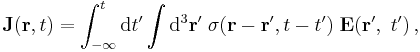
$\mathbf{J} (\mathbf{r}, t) = \int_{-\infty}^t \mathrm{d}t' \int \mathrm{d}^3\mathbf{r}' \; \sigma(\mathbf{r}-\mathbf{r}', t-t') \; \mathbf{E}(\mathbf{r}',\ t') \, ,$

indicating the lag in response by the time dependence of σ, and the non-local nature of response to the field by the spatial dependence of σ, both calculated in principle from an underlying microscopic analysis, for example, in the case of small enough fields, the linear response function for the conductive behavior in the material. See, for example, Giuliani or Rammer.^[3]^[4] The integral extends over the entire past history up to the present time.

As some reflection might indicate, the above conductivity and its associate current density reflect the fundamental mechanisms underlying charge transport in the medium, both in time and over distance.

A Fourier transform in space and time then results in:

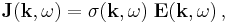
$\mathbf{J} (\mathbf{k}, \omega) = \sigma(\mathbf{k}, \omega) \; \mathbf{E}(\mathbf{k}, \omega) \, ,$

where σ(k, ω) is now a complex function.

In many materials, for example, in crystalline materials, the conductivity is a tensor, and the current is not necessarily in the same direction as the applied field. Aside from the material properties themselves, the application of magnetic fields can alter conductive behavior.

Current through a surface

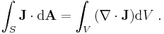
The current through a surface area S perpendicular to the flow can be calculated using a surface integral:

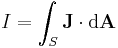
$I=\int_S{ \mathbf{J} \cdot \mathrm{d}\mathbf{A}}$

where the current is in fact the integral of the dot product of the current density vector and the differential of the directed surface element dA, in other words, the net flux of the current density vector field flowing through the surface S.

Continuity equation

Main article: Continuity equation

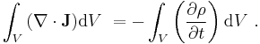
Because charge is conserved, the net flow out of a chosen volume must equal the net change in charge held inside the volume:

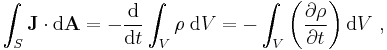
$\int_S{ \mathbf{J} \cdot \mathrm{d}\mathbf{A}} = -\frac{\mathrm{d}}{\mathrm{d}t} \int_V{\rho \; \mathrm{d}V} = - \int_V{\left( \frac{\partial \rho}{\partial t} \right) \mathrm{d}V}\ ,$

where ρ is the charge density per unit volume, and dA is a surface element of the surface S enclosing the volume V. The surface integral on the left expresses the current outflow from the volume, and the negatively signed volume integral on the right expresses the decrease in the total charge inside the volume. From the divergence theorem,

$\int_S{ \mathbf{J} \cdot \mathrm{d}\mathbf{A}} = \int_V{(\mathbf{\nabla} \cdot \mathbf{J}) \mathrm{d}V}\ .$

Hence:

$\int_V{(\mathbf{\nabla} \cdot \mathbf{J}) \mathrm{d}V}\ = - \int_V{\left( \frac{\partial \rho}{\partial t} \right) \mathrm{d}V}\ .$

Because this relation is valid for any volume, independent of size or location,

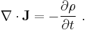
$\nabla \cdot \mathbf{J} = - \frac{\partial \rho}{\partial t}\ .$

This relation is called the continuity equation.^[5]^[6]

In practice

In the domain of electrical wiring (isolated copper), maximum current density can vary from 4A/mm² for a wire isolated from free air to 6A/mm² for a wire in free air. However, for compact designs (e.g. windings of SMPS transformers) the value might be as low as 2A/mm².^[7] If the wire is carrying high frequency currents, depending on its diameter, the skin effect may affect the distribution of the current across the section by concentrating the current on the surface of the conductor. This skin effect plays an important role in Switched-mode power supply transformers where the wires carries high currents and high frequencies (between 10 kHz and 1 MHz). Often in those transformers, the windings are made of multiple isolated wires in parallel with a diameter twice the skin depth and which are twisted together to increase the total skin area and to reduce the impact of the skin effect.

In the domain of printed circuit boards, for TOP and BOTTOM layers, maximum current density can be as high as 35A/mm² with a copper thickness of 35 µm. Inner layers cannot dissipate as much power as outer layers; thus it is not a good idea to put high power lines in inner layers.

In the domain of semiconductors, the maximum current density is given by the manufacturer. A common average is 1mA/µm² at 25°C for 180 nm technology. Above the maximum current density, apart from the joule effect, some other effects like electromigration appear in the micrometer scale.

In biological systems, ion channels regulate the flow of ions (for example, sodium, calcium, potassium) across the membrane in all cells. Current density is measured in pA/pF (picoamperes per picofarad), that is, current divided by capacitance, a de facto measure of membrane area.

In gas discharge lamps, such as flashlamps, current density plays an important role in the output spectrum produced. Low current densities produce spectral line emission and tend to favor longer wavelengths. High current densities produce continuum emission and tend to favor shorter wavelengths.^[8] Low current densities for flash lamps are generally around 1000A/cm². High current densities can be more than 4000A/cm².

References

^ Richard P Martin (2004). Electronic Structure:Basic theory and practical methods. Cambridge University Press. ISBN 0521782856. http://books.google.com/books?id=dmRTFLpSGNsC&pg=PA316&dq=isbn=0521782856#PPA369,M1.
^ Alexander Altland & Ben Simons (2006). Condensed Matter Field Theory. Cambridge University Press. ISBN 9780521845083. http://books.google.com/books?id=0KMkfAMe3JkC&pg=RA4-PA557&dq=isbn=9780521845083#PRA2-PA378,M1.
^ Gabriele Giuliani, Giovanni Vignale (2005). Quantum Theory of the Electron Liquid. Cambridge University Press. p. 111. ISBN 0521821126. http://books.google.com/books?id=kFkIKRfgUpsC&pg=PA538&dq=%22linear+response+theory%22+capacitance+OR+conductance#PPA111,M1.
^ Jørgen Rammer (2007). Quantum Field Theory of Non-equilibrium States. Cambridge University Press. p. 158. ISBN 0521874998. http://books.google.com/books?id=A7TbrAm5Wq0C&pg=PR6&dq=%22linear+response+theory%22+capacitance+OR+conductance#PPA158,M1.
^ Tai L Chow (2006). Introduction to Electromagnetic Theory: A modern perspective. Jones & Bartlett. pp. 130–131. ISBN 0763738271. http://books.google.com/books?id=dpnpMhw1zo8C&pg=PA153&dq=isbn=0763738271#PPA204,M1.
^ Griffiths, D.J. (1999). Introduction to Electrodynamics (3rd Edition ed.). Pearson/Addison-Wesley. p. 213. ISBN 013805326X.
^ A. Pressman et al., Switching power supply design, McGraw-Hill, ISBN 978-0-07-148272-1, page 320
^ Xenon lamp photocathodes

External links

A short explanation of the current density